James S. Martin, Sharon Eve Sonenblum, and Stephen H. Sprigle
Rehabilitation Engineering and Applied Research Laboratory, Georgia Institute of Technology
Introduction
Pressure ulcers are a major problem for wheelchair users [ ]. Pressure ulcer prevention typically involves the use of a pressure-distributing wheelchair cushion and/or by periodic pressure relief (PR) or weight shift activities performed by the subject [ ]. In order to gauge the efficacy of these PRs in preventing pressure ulcers, it is necessary to compile a record of their nature and frequency under realistic in-situ conditions. Additionally, it is necessary that this record be accomplished by a non-intrusive objective measurement system. This insures that the subject’s behavior is not influenced by the data collection and that PRs that are both volitional and those that are incidental to daily activities are properly recorded.
A previous paper describes a pressure relief monitoring sensor mat (PRM) that was developed for these measurements [ ]. The mat is located between the cushion and the seat of a chair so that its presence does not affect cushion performance. In this location, the measured pressures are not as easily interpretable as they would be if they were measured by an interface pressure mat (IPM) located between the buttocks and the cushion. This is because the cushion redistributes loading between the buttocks and the PRM and because it introduces latency into the pressure measured at this location relative to the interface pressure. Thus, a more complex algorithm is required to determine the instantaneous PR status than would be needed to analyze IPM data. Furthermore, both IPM and PRM data, when collected over many hours, experience creep effects that make identifying PR’s more challenging.
Previous efforts to develop an algorithm for determining instantaneous PR status were successful when tested in laboratory conditions, but highly over-reported PRs when applied to real-world data. Therefore, the goal of this study was to develop an improved algorithm for detecting PRs based on PRM data collected in real-world conditions.
processor description
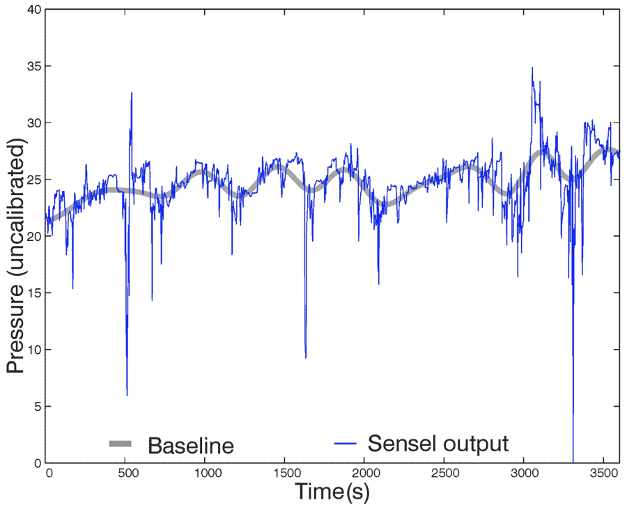 Figure 1: Comparison of sensel output and computed baseline for the left posterior lateral sensel.
The PRM contains 8 distinct sensels, which provide pressure information for 8 locations on a rectangular grid. Four of these sensels are under the right buttock and four are under the left. In each of these subgroups there are two medial and two lateral sensels that are in parallel anterior/posterior locations. All PRs must be measured with respect to a baseline (loaded) condition. Finding the baseline condition for each sensel in the PRM is the first step in the processor.
As a subjects is apt to reposition himself in his chair, the baseline condition is time-dependent, but represents a slower change than that associated with PR activities. It is therefore determined by low-pass filtering the measured pressure from each sensel. This filter is implemented in two steps. In the first of these, periods of zero pressure, are removed from the sensel data. These may represent either PRs or time that the subject was out of the chair, but are clearly not indicative of a baseline condition. In the second step a four-pole butterworth low-pass filter with a cutoff period of 200 seconds (i.e. 1/200 Hz) was implemented acausally using the filtfilt function in Matlab , which applies the filter both forward and backward in time. This insured that, despite the very low frequency of the filter, the computed baseline was not delayed with respect to the data. This result was then interpolated linearly across the periods of time corresponding to the measured zero pressures so that there was a one to one correspondence between the baseline set and the data set. A representative period of data and the corresponding computed baseline is shown in figure 1.
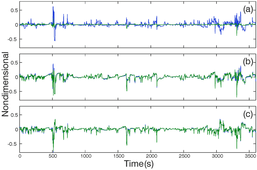 Figure 2: Features used for classification: (a) features used for both left and right PR classification, (b) features used for right PR classification only, and (c) features used for left PR classification only
In the second step of the processing, representative features are extracted from the data and normalized by the computed baseline values. This reduces the dimensionality of the data set from the 8 sensel values to six features. The features are:
- Center of Pressure Anterior-Posterior - the coordinates of the measured center of pressure in the anterior-posterior direction, normalized as the distance from the baseline location
- Center of Pressure Medial-Lateral - the coordinates of the measured center of pressure in the medial-lateral direction, normalized as the distance from the baseline location
- Total Pressure Left or Right – Total pressure measured by the 4 sensels on the left or right (respectively), divided by the baseline value
- Average Pressure Left or Right – Average pressure measured by the 4 sensels on the left or right (respectively), divided by the baseline value
The centers of pressure are relevant to the PR status of both the right and the left buttock. The total and average pressures on the left and right are used for determining the PR status on the respective sides. Thus there is a set of four features used to evaluate the PR status of each buttock, which is carried out independently other than that there is overlap between these sets. Overall PR status will be defined as either buttock experiencing PR. Figure 2 depicts the features corresponding to the raw data and baseline depicted in figure 1.
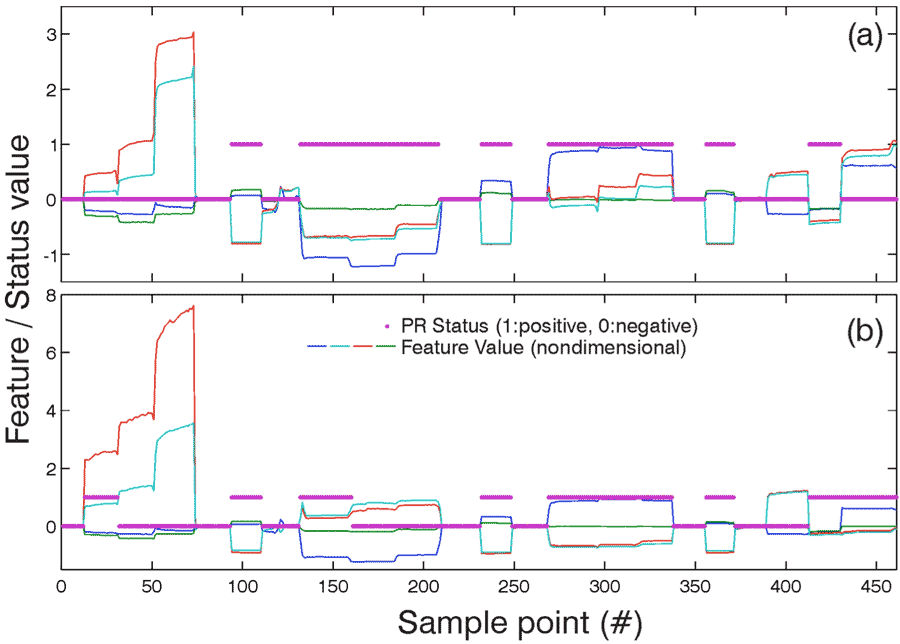 Figure 3: Classifier training sets. (a) right and (b) left
In the third step of the processing, PRM data from an initial training set is compared with ground truth data collected from an IPM. During this data collection the subject was instructed to perform a series of maneuvers including differing degrees of leans to his right, left, and forward along with full lifts against the arms of his chair. Each maneuver is assigned a PR status based on the IPM data, which was thus associated with the concurrent PRM features. This set of feature-status pairs represents a classifier that can be used to evaluate the remaining data for which no IPM measurement is available. A typical training set/classifier is depicted in figure 3.
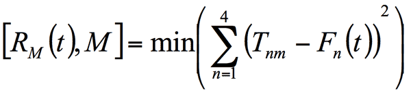
The classifier was implemented using Euclidean nearest neighbors to separately determine the PR status of the right and left buttocks [ ]. The distance between each data point in the relevant 4-dimensional feature space and all of the known points in the classifier set is computed. The known point corresponding to the minimum of the resulting array of computed distances is then assumed to represent the PR status of the data point. This may be represented as:
 |
(1) |
and
S(t) = S![]() M
M
Where T![]() nm is the nth feature of the mth point in the classifier training set, F
nm is the nth feature of the mth point in the classifier training set, F![]() n is the nth feature of the data, R
n is the nth feature of the data, R![]() M is the distance in feature space between the data point and its nearest classified neighbor, M is the index of that neighbor in the training set, and S
M is the distance in feature space between the data point and its nearest classified neighbor, M is the index of that neighbor in the training set, and S![]() M is the corresponding PR status with positive indicating a potential PR and negative (or null) indicating otherwise.
M is the corresponding PR status with positive indicating a potential PR and negative (or null) indicating otherwise.
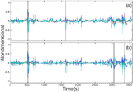 Figure 4: Classified data. (a) right buttock features and classifications, (b) left buttock features and classifications. Gray bands indicate PRs
The instantaneous PR status, which is represented by S(t) in equation 1, is not sufficient to determine a PR by itself. If a positive status is particularly short in duration, it is more likely to be noise than an actual PR. The body has considerable inertia which limits the speed with which movements will occur. Similarly, a positive status on both buttocks that is recorded for a relatively long period is likely to be representative of the subject being out of the chair, as maintaining a complete PR for an extended time is difficult. In this case his actual PR status is unknown, as he may be performing an extended PR, experiencing PR by laying in side-lying or another posture, or simply seated on a different surface. These two cases are handled specifically. If a positive status is not part of a contiguous positive period that is at least 5s in duration, it is deemed to be negative. If a positive status is part of a contiguous positive period of 60s or longer that is concurrent with a similar period on the opposite buttock, it is deemed to be unknown. An example of the results of this processing along with the normalized features that were used for the evaluation are depicted in figure 4. During the one-hour period of data shown, the subject exhibibitted 6 PRs. Two of these were total PRs apparent on both buttocks. One was a right PR only. Two were left PRs only.
Processor limitations
The accuracy of the processor is dependent on several aspects of the data set. Baseline determination may be skewed by excessive activity of the subject for a prolonged period, the inadvertent inclusion of PRs in the computation, or an inappropriate selection of low-pass filter cutoff frequency for a particular subject’s typical activities. As the current parameters and methods have not yet been tested on a large number of subjects, it is difficult to quantify these effects.
The nearest-neighbor classifier that was used has two potential shortcomings in that it is strongly dependent on both the accuracy and the distribution of data in the training set. Inaccurate training-set status values can have a profound effect on the accuracy of the classifier, regardless of their number. The magnitude of this effect depends entirely on the distribution of errant results in the 4-dimensional feature space. To the extent that a bad value stands apart from any other clusters of values in this space, it is likely to constitute a nearest neighbor for more of the data that is distributed through that space than an element of any cluster whose omission would have a minimal effect on the results. The problem that this poses is further compounded by the fact that a bad training set value need not represent a data collection error. The latency and pressure redistribution associated with the intervening cushion may mean that PRM data that is concurrent with a correctly evaluated IPM status poorly characterizes that PR status. This is a likely scenario during transitions between a positive and negative PR status. Currently, this problem is dealt with by manually inspecting the training set data and correcting or culling problematic elements.
The second potential problem with the classifier relates to the distribution of data in the training set. If the set must define a region of PR status with the feature space that is topographically complex or non-contiguous, then many more distinct elements are required for the set to constitute a robust classifier. This problem is illustrated in figure 5, which depicts training set values viewed in three dimensions of the parameter space. It is apparent from the figure that the spatial regions linking the clusters of data points, which should exist if regions of uniform status are contiguous, are void of information. Thus the classification of data points in these regions carries significantly more uncertainty that the classification of points that lay close to the training set clusters. There is no mathematical requirement that regions of uniform status be contiguous, however this is intuitive based on the observation that a transition between different subject orientations defined as PR should not require the subject to pass through a PR-negative state.
Conclusions
Work on the signal processor described in this paper is ongoing. The values and techniques that it makes use of will evolve and adapt as it is applied to a greater volume of subject data. Data collection will, in turn, be informed by the needs of the classifier. In particular, initial results have demonstrated the value of a more expansive training data set as is apparent in scattering of training values in figure 5a; the possibility of reducing the dimensionality of the feature set used for classification as is apparent from the near-colinearity of training values in figure 5b; and the importance of properly determining a moving baseline from measured data. Initial results have also suggest that subject activity may be determined from a single variable: the total path length traversed in the feature space over a specified period of time
References
- Krause J.S. and Broderick L. (2004). Patterns of recurrent pressure ulcers after spinal cord injury: identification of risk and protective factors 5 or more years after onset. Archives of Physical Medicine and Rehabilitation vol.85 pp. 1257-1264.
- Bain D.S. and Ferguson-Pell, Remote monitoring of sitting behavior of people with spinal cord injury. (2002). Journal of Rehabilitation Research and Development Vol. 39 pp 513-520.
- Dai, R., Sonenblum, S.E., and Sprigle,S. (2012). A Robust Wheelchair Pressure Relief Monitoring System. Annual International Conference of the IEEE Engineering in Medicine and Biology Society (EMBC), p 6107-10.
- Mathworks Matlab documention (2014). Retrieved January 14, 2014 from http://www.mathworks.com/help/signal/ref/filtfilt.html?searchHighlight=filtfilt
- Weisstein, E.W. (1999) CRC concise Encyclopedia of Mathematics.Chapman and Hall, NY. Pg. 1220.
Acknowledgements
This work was funded by the National Institute on Disability and Rehabilitation Research of the U.S. Department of Education under grant number H133E080003.
Audio Version PDF Version